Merge Sort, Divide & Conquer, Master Theorem

Class Material

• Slides can be found here.

---

Notations: Big-O vs. Little-o

In computational complexity theory, Big-O (denoted as $O(\cdot)$) and Little-o (denoted as $o(\cdot)$) are both used to describe the growth rates of functions, but they differ subtly in how tightly they bound the growth of one function relative to another. Below is a detailed comparison between the two:

---

Big-O Notation (O)

• Definition: $f(n) \in O(g(n))$ means that f(n) does not grow faster than g(n) up to a constant factor for sufficiently large n.

  • There exist positive constants $C$ and $n_0$ such that: $f(n) \leq C \cdot g(n) \quad \text{for all} \quad n \geq n_0$

• Intuition:
  Big-O provides an upper bound on the growth rate of $f(n)$. It tells us that $f(n)$ grows at most as fast as $g(n)$ asymptotically. It allows equality — meaning $f(n)$ and $g(n)$ could potentially grow at the same rate.

• Example:
  $2n^2 + 3n + 5 \in O(n^2)$ because, asymptotically, $n^2$ is the dominant term (the other terms grow more slowly). So $2n^2 + 3n + 5$ does not grow faster than $n^2$.

---

Little-o Notation (o)

• Definition: $f(n) \in o(g(n))$ means that f(n) grows strictly slower than g(n), even without any constant factor.

  • Formally, for every positive constant $C$, there exists $n_0$ such that: $f(n) < C \cdot g(n) \quad \text{for all} \quad n \geq n_0$
  • This implies that the ratio $f(n) / g(n) \to 0$ as $n \to \infty$.

• Intuition:
  Little-o provides a strict upper bound on the growth rate. It says that $f(n)$ grows strictly slower than $g(n)$ as $n$ becomes large, and they cannot grow at the same rate.

• Example:
  $n \in o(n^2)$ because $n$ grows slower than $n^2$ as $n \to \infty$. Specifically, the ratio $n / n^2 = 1/n \to 0$.

  $n^2 \notin o(n^2)$ because $n^2$ grows at the same rate as $n^2$ (not strictly slower). The ratio $n^2 / n^2 = 1$ as $n \to \infty$. (We don't need to use L'Hôpital's Rule because it is not an indeterminate form – both the numerator and denominator grow at the same rate. Since they are identical, their ratio is always 1, no matter how large $\frac{n}{n}$ becomes.)

Application of L'Hôpital's Rule in asymptotic analysis

The expression $\frac{\infty}{\infty}$ (infinity over infinity) is considered an indeterminate form in calculus. This means it is not immediately clear what the value should be, and further analysis is required to evaluate it properly.

---

Why is $\frac{\infty}{\infty}$ Indeterminate?

• Infinity ($\infty$) is a concept, not a real number. It indicates that a value grows without bound.
• When we encounter $\frac{\infty}{\infty}$, both the numerator and the denominator are growing indefinitely, but we don’t know how fast they grow relative to each other. Depending on the functions involved, the ratio could result in different outcomes:
  • Finite value: $\frac{n}{2n} \to \frac{1}{2}$ as $n \to \infty$.
  • Infinity: $\frac{n^2}{n} \to \infty$ as $n \to \infty$.
  • Zero: $\frac{n}{n^2} \to 0$ as $n \to \infty$.

---

Resolving $\frac{\infty}{\infty}$ using L'Hôpital's Rule

When a limit yields the form $\frac{\infty}{\infty}$, we often apply L'Hôpital's Rule to evaluate it. L'Hôpital’s Rule states:

$$\lim_{x \to \infty} \frac{f(x)}{g(x)} = \lim_{x \to \infty} \frac{f'(x)}{g'(x)},$$

provided that both $f(x) \to \infty$ and $g(x) \to \infty$, and the derivatives $f'(x)$ and $g'(x)$ exist.

---

Example Using L'Hôpital's Rule

Evaluate:

$$\lim_{x \to \infty} \frac{x}{e^x}.$$

Both the numerator $x$ and the denominator $e^x$ go to infinity, giving $\frac{\infty}{\infty}$. Applying L'Hôpital's Rule:

$$\lim_{x \to \infty} \frac{x}{e^x} = \lim_{x \to \infty} \frac{1}{e^x} = 0.$$

---

Summary

$\frac{\infty}{\infty}$ is indeterminate because it can lead to different results depending on the growth rates of the functions involved. To resolve it, we need more information, often using tools like L'Hôpital's Rule or algebraic manipulation.

---

Key Differences between Big-O and Little-o

Aspect	Big-O (O)	Little-o (o)
Bound Type	Upper bound (not strict)	Strict upper bound
Equality Allowed?	Yes (same growth rate possible)	No (strictly slower growth)
Mathematical Limit	$\lim_{n \to \infty} f(n) / g(n) \leq \infty$	$\lim_{n \to \infty} f(n) / g(n) = 0$
Example Relationship	$n^2 \in O(n^2)$	$n \in o(n^2)$

---

Summary

• Big-O notation allows for equal growth rates (or $f(n)$ can grow slower or at the same rate as $g(n)$).
• Little-o notation requires that $f(n)$ grows strictly slower than $g(n)$.
  Both notations are useful tools in asymptotic analysis to describe how algorithms perform as input sizes grow large.

In asymptotic analysis, $n_0$ is the threshold beyond which the behavior of the function we’re analyzing matches the specified growth bound. Essentially, it marks the point where the asymptotic relationship becomes valid.

---

Role of $n_0$ in Asymptotic Notations

• When we say that $f(n) \in O(g(n))$, it means that after a certain input size $n \geq n_0$, the inequality holds: $$f(n) \leq C \cdot g(n) \quad \text{for all} \quad n \geq n_0$$
• For little-o notation $f(n) \in o(g(n))$, the idea is that for all positive constants $C$, there exists an $n_0$ beyond which: $$f(n) < C \cdot g(n) \quad \text{for all} \quad n \geq n_0$$

Intuition

• $n_0$ ensures that the asymptotic behavior is true only for large enough input sizes. For smaller values $n < n_0$, the functions may behave unpredictably, but asymptotic notations focus on large $n$.

---

Example

Say we claim that $f(n) = 3n + 2 \in O(n)$.

• For small $n$, the $+2$ term might dominate. However, for large enough $n$, $3n + 2$ behaves similarly to $3n$.
• In this case, $n_0$ would be the point where $3n + 2 \leq C \cdot n$ for some constant $C$. For example, with $C = 4$, we can say that the inequality holds for $n \geq n_0 = 2$.

---

Summary

• $n_0$ is the starting point beyond which the asymptotic bound (like $O(g(n))$ or $o(g(n))$) reliably holds.
• Asymptotic notations don't care about small inputs—only what happens as $n \to \infty$ matters. $n_0$ ensures that we focus on that asymptotic behavior.

---

Sorting Algorithms

Merge Sort

Resources

• Why is Merge Sort $O(n \log n)$?

Lemma: No sorting algorithm can sort $n$ arbitrary numbers in $o (n \log n)$ comparisons

• This means that Merge Sort is optimal in terms of the number of comparisons it makes.

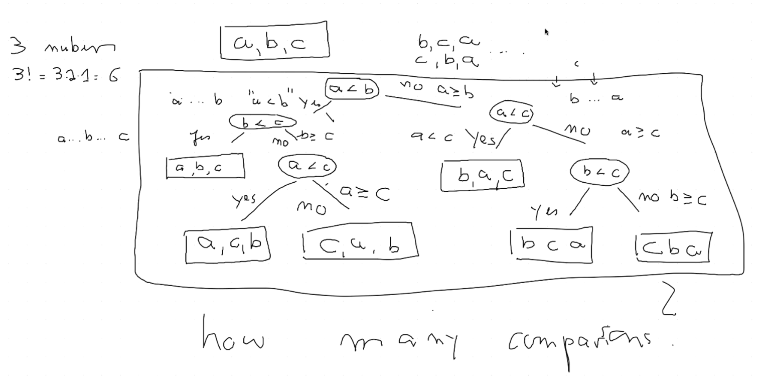
Comparison Trees

In the slides: Using Comparison Trees to describe any comparison-based algorithm.

• The height of the tree represents the number of comparisons made by the algorithm: $\log(n)$.

  To arrive at a specific leaf, which is the correct result – a sorted permutation, we've only had to traverse at worst the max height of the tree.

• The number of leaves represents the number of possible outcomes: $n!$. (For example: $\{a, b, c\}$ has $3!$ possible permutations)

Note

• These assume that the tree is a binary tree.
• Comparisons have exactly 2 results: "$a < b$" or "$a >= b$".

Showing that Comparison Trees are $\Omega(n \log n)$

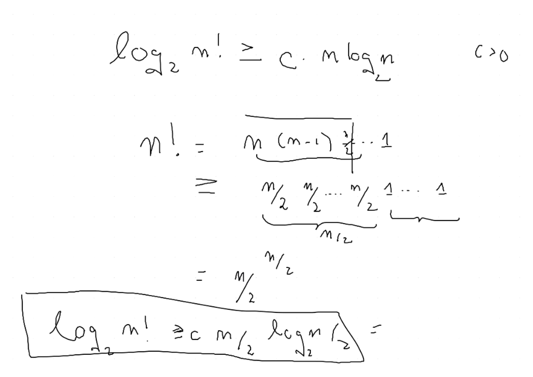
To show that $\log_2(m!)$ is $\Omega(n \log n)$ without using Stirling's approximation, we need to lower bound $\log_2(m!)$ and compare it asymptotically with $n \log n$.

---

Step 1: Express $\log_2(m!)$

We start with the definition of the factorial's logarithm:

$$\log_2(m!) = \log_2(1 \cdot 2 \cdot 3 \cdots m).$$

Using the logarithm of a product:

$$\log_2(m!) = \log_2(1) + \log_2(2) + \log_2(3) + \cdots + \log_2(m).$$

---

Step 2: Lower Bound $\log_2(m!)$

Notice that the sum $\log_2(1) + \log_2(2) + \cdots + \log_2(m)$ can be lower-bounded by focusing on the second half of the terms (those from $m/2$ to $m$):

$$\log_2(m!) \geq \sum_{k = m/2}^m \log_2(k).$$

Tip: We can do this magic step of focusing on the second half because of the "$\geq$" sign. We're looking for a lower bound, so we can ignore the first half of the terms. For graphical intution, the prof's half-baked example here might help, though it is not entirely complete.

Since for all $k$ in this range, $k \geq m/2$, we can lower bound each $\log_2(k)$ by $\log_2(m/2)$:

$$\log_2(m!) \geq \sum_{k = m/2}^m \log_2\left(\frac{m}{2}\right).$$

There are $m - m/2 + 1 = m/2 + 1$ terms in this sum, so:

$$\log_2(m!) \geq \left(\frac{m}{2} + 1\right) \log_2\left(\frac{m}{2}\right).$$

---

Step 3: Simplify the Lower Bound

We simplify the expression $\left(\frac{m}{2} + 1\right) \log_2\left(\frac{m}{2}\right)$. For large $m$, the term $+1$ is insignificant, so:

$$\log_2(m!) \geq \frac{m}{2} \log_2\left(\frac{m}{2}\right).$$

Using $\log_2\left(\frac{m}{2}\right) = \log_2(m) - \log_2(2) = \log_2(m) - 1$, we get:

$$\log_2(m!) \geq \frac{m}{2} \left(\log_2(m) - 1\right).$$

For large $m$, the $-1$ becomes negligible, so:

$$\log_2(m!) \geq \frac{m}{2} \log_2(m).$$

---

Step 4: Compare with $n \log n$

Now we want to compare $\log_2(m!)$ with $n \log n$. If we set $m = n$, the lower bound becomes:

$$\log_2(n!) \geq \frac{n}{2} \log_2(n).$$

This shows that $\log_2(n!)$ grows asymptotically at least as fast as $\frac{n}{2} \log_2(n)$, which is clearly $\Omega(n \log n)$. Therefore:

$$\log_2(m!) = \Omega(n \log n).$$

---

Conclusion

We have shown that $\log_2(m!)$ is $\Omega(n \log n)$ without using Stirling’s approximation by directly analyzing a lower bound of the sum $\log_2(1) + \log_2(2) + \cdots + \log_2(m)$.

Master Theorem

Resources

• What is Master Theorem
• Proof of Master Theorem

Aside

• If you're having a hard time understanding the proof for Master Theorem, watching the Merge Sort video first will 100% help.